
Simulation of Coating-Film Drying : A Practical Introduction to 1D/3D Analysis for Coating, Painting, and Electrode Processes
1.Introduction
In manufacturing fields such as automotive painting, secondary-battery electrodes, and functional films, "coating and drying" is an essential process step. However, drying is not simply "removing solvent". During drying, multiple changes progress simultaneously inside the coating film. Therefore, when issues such as surface whitening, cracks after drying, or delamination from the substrate occur, understanding component transport and phase separation inside the film during drying often provides the most direct path to troubleshooting. This article explains mechanisms of coating-film drying that are difficult to observe by experiments alone, and introduces simulation-based approaches to analyze them.
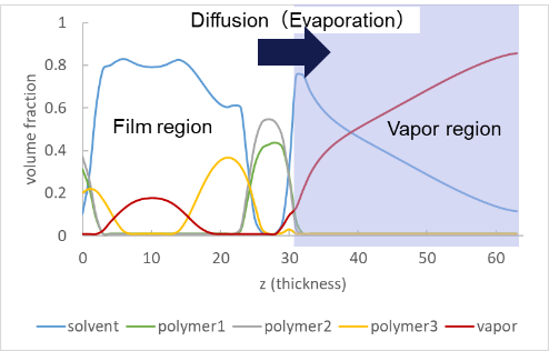
Although a typical coating film is only a few micrometers to a few hundred micrometers thick, significant changes occur inside it. A particularly important aspect is the concentration profile along the thickness direction (the Z direction) created during drying. As solvent evaporates from the surface, solids in the formulation (resins, binders, particles, etc.) redistribute under the competing effects of the following two mechanisms[1–4,11]:
- Advection: a flow that carries components along with the solvent as it leaves from the surface
- Diffusion: motion that reduces concentration gradients and tends to homogenize the composition
The balance between these mechanisms can lead to a range of phenomena, including skin-layer formation and component segregation.
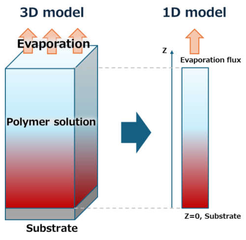
2.Selecting an Appropriate Model
When performing simulations, it is not always necessary to model every phenomenon in a detailed three-dimensional setting. It is important to choose an appropriate model based on the characteristics of the phenomenon.
(1) Cases where a 3D model is required
3D model is effective when micrometer-scale (or smaller) fine structures (domains) form in the in-plane direction of the film. Examples include:
- Functional films where intentional phase separation is used to create sea–island or co-continuous structures
- Situations where strong in-plane flows (e.g., Marangoni convection) are induced by temperature or concentration nonuniformity during drying
These cases, including those where one wants to examine microscopic behavior of filler dispersion structures during evaporation, cannot be represented by a thickness-only 1D model. In such situations, 3D analysis becomes important[5,6,9,12,13].
(2) Cases where a 1D model is effective
On the other hand, 1D model is highly effective in cases such as:
- A wide coated area where the in-plane direction can be regarded as nearly uniform
- Cases where the suspected root cause is mainly "concentration nonuniformity along the film thickness"
In such cases, extracting only the thickness direction (Z direction) from a wide coated area can substantially reduce computational cost while still capturing the essential physics of component transport and phase separation.
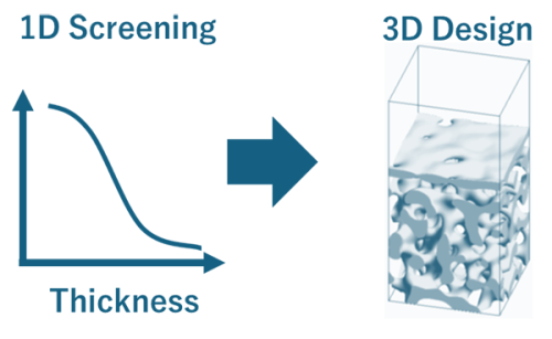
3.Why 1D Simulation Is Often a Practical First Step
A key reason that starting with a 1D model is realistic in many cases is the difference in time scales. The time t required for diffusion is proportional to the square of the transport length L, and can be roughly expressed as t ~ L2 / D, where D is the diffusion coefficient. Because the thickness direction (tens to hundreds of micrometers) and the in-plane direction (millimeters to centimeters) differ in order of magnitude, diffusion along the in-plane direction requires orders of magnitude longer time even for the same D.
For a typical polymer solution (depending on conditions), if we assume D ~ 10-10~10-11 [m2/s], a very rough estimate using the above expression suggests:
- Diffusion across the thickness direction (tens to hundreds of micrometers): proceeds on a relatively short time scale (seconds to minutes)
- Diffusion along the in-plane direction (millimeters to centimeters): requires much longer time scales (hours to days)
Therefore, within the time scale of typical drying processes, it is often reasonable to treat the in-plane direction as "almost stationary."
Leveraging this, it is efficient to first evaluate thickness-direction behavior quickly using a 1D model, screening conditions such as temperature, film thickness, and solvent type, and then, as needed, expand to a 3D model. This hierarchical approach is often practical.
4."Drying Speed" vs. "Mixing Speed"
A useful indicator for interpreting thickness-direction concentration profiles in a 1D model is the Péclet number (Pe). Pe represents the ratio of drying speed (the apparent speed associated with film shrinkage) to mixing speed (diffusion).
Conceptually: Pe ∼(apparent transport speed due to drying) / (ease of mixing by diffusion)
- Intuitively:
-
- Large Pe (rapid drying)
- Drying (solvent removal) is much faster than diffusion, so the surface becomes increasingly concentrated before components can fully mix. As a result, a skin layer forms more easily, and the risk of surface hardening and solvent retention inside the film increases.
- Small Pe (slow drying)
- Diffusion can "keep up" with drying, so components tend to remain more uniform along the thickness direction. These conditions are more likely to yield a homogeneous coating film.
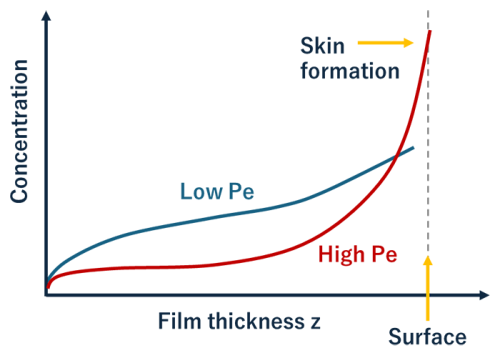
When Pe is large, solute concentration becomes high near the surface, leading to skin-layer formation.
Pe is useful as an axis for quantitatively comparing how "high-Pe-like" or "low-Pe-like" different drying conditions are (temperature, atmosphere, film thickness, etc.). This provides a common basis for discussion across processes such as painting, electrode coating, and film formation.
5.Application Examples by Industry
The above concepts and simulation approaches can be applied in a wide range of product development contexts.
(1) Automotive painting
In automotive painting, issues such as loss of gloss, whitening, cracking, and poor adhesion are often challenges. These phenomena are considered to be related to internal film structure, especially the distribution of components and structure along the thickness direction. An important theme is therefore how to "design where each component should reside."
By using experimental data together with simulation results, one can examine formulations and drying conditions that lead to a desired internal structure. For example, simulations have been applied toward realizing composition/functionally graded structures within a single painting process, such as increasing acrylic resin near the film surface for weather resistance and increasing epoxy resin near the substrate interface where corrosion resistance and adhesion are important[7,8].
(2) Battery electrodes
In electrode manufacturing for lithium-ion batteries and related systems, segregation of binder components can be an issue. Under higher-temperature drying conditions, it has been reported that binders and conductive additives migrate toward the surface, leading to a thickness-direction bias in which their amounts are relatively reduced near the current collector (substrate)[10]. Such bias may adversely affect mechanical and electrical properties of the electrode.
It has also been discussed that, using a 1D model, binder concentration profiles along the thickness direction during drying can be tracked over time and the influence of drying speed can be analyzed[11]. For example, one can use a 1D model to predict binder concentration near the current-collector interface and assess how far the drying rate can be increased before the risk of defects becomes significant.
For more detailed mechanism analysis, such as explicitly treating fine particles, 3D models are applied. Depending on the target scale, examples include coarse-grained molecular dynamics and particle-based methods built on continuum models[5,6]. The intent is to use such simulation results as input for screening drying conditions and setting process windows.
(3) Functional membranes
In porous membranes such as filters, porous structures are formed via phase separation associated with drying or solvent exchange. Phase separation occurring within the film during evaporation can change the final structure depending on its timing and rate. Therefore, when needed, evaluating phase-separation patterns and domain size (pore size) using a 3D Phase-Field model is effective[12,13].
By first checking the time relationship among evaporation, diffusion, and phase separation using a 1D model, then narrowing to key conditions before moving to 3D analysis, it becomes easier to balance computational cost with depth of design exploration.
6.Applying Simulation Software
To handle complex physical phenomena such as evaporation, diffusion, fine-particle dispersion, phase separation, and skin formation, J-OCTA provides multiple simulation methods. It is important to understand the characteristics of each method and the spatial scale it targets. Recently, linkage with machine learning is also of interest; by learning from simulation results, it may become possible to use them for faster prediction.
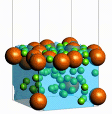
- (Coarse-grained) molecular dynamics : spatial scale roughly 10 nm to 100 nm
- Enables microscopic analysis that can treat interactions between fillers and molecules in detail.
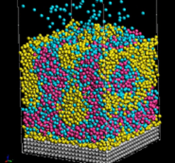
As the solvent (blue) evaporates, polymers (red, yellow) form a phase-separated structure.
- Dissipative particle dynamics (DPD) : spatial scale roughly 10 nm to 1 μm
- Used to analyze phase-separation dynamics including fillers, while also considering hydrodynamic effects.
- Mean-field methods (Phase-Field, SCFT) : spatial scale roughly 10 nm to 10 μm
- Used to analyze phase-separated structures. A 3D model can resolve detailed microstructures, while a 1D model can be applied to larger scales. Coupling with flow-field analysis is also possible.
- Fluid analysis based on continuum models (e.g., particle methods) : spatial scale roughly 100 nm to 100 μm
- Although this no longer uses a molecular description, it can analyze larger-scale behavior such as flow fields in filler dispersions.
As solvent evaporates, particles of different sizes form a connected structure.
7.Summary
In coating-film drying processes, it is important to understand "what is happening inside the film while it is drying". When using simulations, it is often effective to take a staged approach: first check thickness-direction component distributions and the presence/absence of skin formation using a 1D model, and then, if necessary, examine fine microstructures in detail using a 3D model. This may reduce experimental trial-and-error and help shorten development cycles.
If you are interested in the topics introduced here, please feel free to contact us.
- Journal of Electrochemical Energy Conversion and Storage, 20, 030801,(2023). https://doi.org/10.1115/1.4055392
- Physical Review Letters, 97, 136103, (2006). https://doi.org/10.1103/PhysRevLett.97.136103
- Japanese Journal of Applied Physics, 45, 8817, (2006). https://doi.org/10.1143/JJAP.45.8817
- Nihon Reoroji Gakkaishi, 39, 17, (2011). https://doi.org/10.1678/rheology.39.17
- Simulation of Solvent Evaporation Using DPD https://www.jsol-cae.com/en/products/j-octa/cases/A026.html
- Simulation of evaporation of liquid film https://www.jsol-cae.com/en/products/j-octa/cases/A073.html
- (in Japanese) "Compositional Gradients in Acrylic/Epoxy Blended Film: Computer Simulation", Kansai Paint, (2006) https://asset.kansai.co.jp/uploads/rd/paint_study/pdf/146/02.pdf
- (in Japanese) "Compositional Gradient in Acrylic/Epoxy Blended Film: Development and Control", Kansai Paint, (2005) https://asset.kansai.co.jp/uploads/rd/paint_study/pdf/143/06.pdf
- Slurry Coating Process [Courtesy of Toyota Motor Corporation] https://www.jsol-cae.com/en/products/j-octa/cases/A036.html
- Journal of Power Sources, 591, 233883, (2024).
https://doi.org/10.1016/j.jpowsour.2023.233883 - Journal of Power Sources, 393, 177, (2018).
https://doi.org/10.1016/j.jpowsour.2018.04.097 - "Simulation of phase separation process in polymeric membranes"
https://www.jsol-cae.com/en/products/j-octa/cases/A062.html - Journal of Membrane Science, 620, 118941, (2021).
https://doi.org/10.1016/j.memsci.2020.118941
Articles in the Same Category
Related Information
Categories
New articles
- Simulation of Coating-Film Drying : A Practical Introduction to 1D/3D Analysis for Coating, Painting, and Electrode Processes
- Designing Plastic Recycling with Molecular Simulation
- What is Materials Informatics (MI)?
Next-generation materials development accelerated by AI × simulation
- Electrical conduction as a multiscale simulation
- Development of force fields used in molecular dynamics calculation
- What you need to know when using molecular modeling and simulation for materials design
- Materials & Process Informatics
- Machine Learning for Materials Design in J-OCTA - - Simulation of lithium-ion batteries
- Drug Discovery and Formulation
- Simulation of Polymeric Materials : Overview and Examples
